When it comes to modern intralogistics, AGVs (Automated Guided Vehicles) have become indispensable. These move goods from A to B without having to be controlled by a human being. To ensure that the vehicles can be seamlessly integrated into the existing process landscape, they should be controlled by a higher-level master control system, ideally via VDA 5050. The master control system has the task of processing the orders that arise, which may come from an ERP system, for example, as efficiently as possible with the available vehicles. But how many vehicles are needed and what number do companies need to acquire for their intended processes?
These questions can be answered by simulating a scenario that is as realistic as possible. The basic idea is that virtual vehicles process a scenario of orders in a highly accelerated simulation, resulting in KPIs on punctuality, utilisation and empty runs. This involves varying the number of vehicles available and comparing the KPIs so that a statement can be made.
AGV Hub with simulation tool brings light into the darkness
Within the AGV Hub of Flexus, which runs on the SAP-BTP, one can make exactly these statements with the simulation add-on. First – as in a normal project – the area is created graphically with the RouteOptimizer. Nodes and edges are set on the customer’s background map and provided with pick-up and delivery stations as well as the routes. The scale of the map is important here so that a realistic result can be calculated in terms of the time required for the routes travelled.
Another input required is the order data, which must be simulated. Depending on the previous system, the data is available in different forms. In the best case, the customer already uses the FlexGuide transport guidance system and can access actual data in live operation. Alternatively, bookings from SAP modules such as WM, EWM or PP could be used to generate the data. Each job has a source and sink and, if applicable, a job type that must be prioritised differently. Thus, supplies for production could be more important than the disposal of empties.
An important point in the simulation is that not all orders are available immediately, but only come into the system gradually, as in daily operations. Therefore, each order should have a creation time when it is available to the system in the (virtual) timeline. In addition, the orders can be enriched with further data:
- Is there a due date when the order must be completed?
- Does the order have a special load carrier type that can only be driven by a special AGV type?
The orders should cover the period of at least one whole working day, better still a whole week, in order to be able to consider fluctuations among the individual days of the week separately.
Set up the simulation: Map real situations
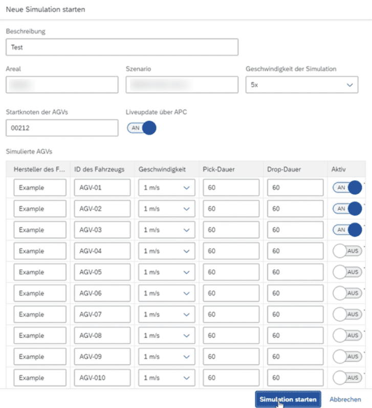
Now the actual simulation can be started. A few parameters still need to be set for this. First, you choose a number of vehicles with which to run the simulation. For each vehicle, the speed, the duration for picking up and the duration for dropping off a job can be set. In addition, the speed of the simulation can be selected.
However, caution must be exercised here: by using the actual MQTT broker for the VDA 5050 messages, the communication time between simulation and MQTT broker plays a role. The higher the speed, the greater the influence of the waiting time on the communication of both systems. Here, a value of “times five” has proven to be a good average.
Let’s start: Simulate real journeys in your warehouse
As soon as the simulation starts, a virtual agent is created for each vehicle, which has the task of simulating the vehicle within the MQTT broker. This means that the agent logs on to the MQTT broker as a participant and receives orders from the control system via it. As soon as it has received the order to drive to the from or to place, it simulates its journey using the route network at the set speed.
The agent continuously reports its X / Y position to the control system as well as the arrival at each intermediate node. The control system in turn now also controls traffic at intersections or dead ends, as in live operation, by releasing nodes for AGVs or refusing to release them because another vehicle is in the corresponding area. The implementation of traffic management is an important point in the simulation, as waiting vehicles at intersections naturally increase travel times, which in turn are reflected in the final results.
The decision as to which vehicle receives which order at which time is made using the same algorithms as in live operation. The customising parameters of the FlexGuide transport control system within SAP are used. These can be used to adjust the weighting between minimising empty runs, keeping due dates as well as possible double plays. This approach is important in order to present the simulation as close to reality and as credible as possible. The use of external simulation tools would follow different rules of allocation and would therefore not have been feasible. Currently, battery management has not been implemented because it is difficult to determine the charging and discharging speed. However, a function has been implemented that directs the AGVs to a predefined loading bay if there are no orders in the pool.
Simulation analysis: These parameters can be optimised at your site in the future
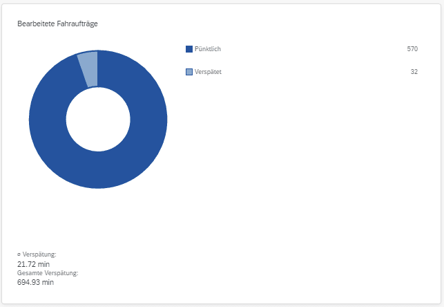
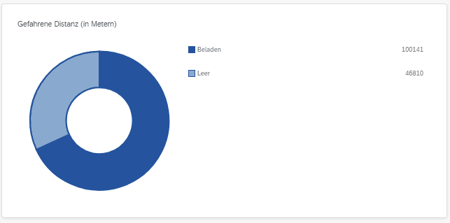
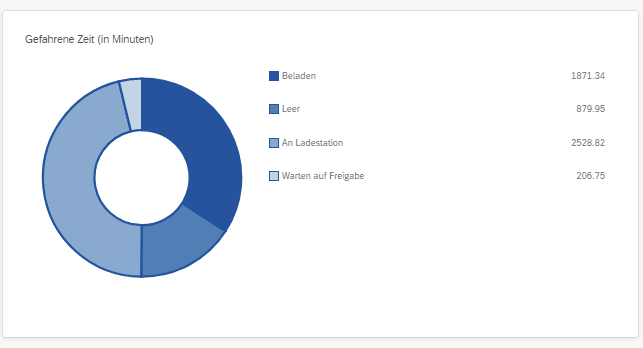
Once the simulation has run, the result is a large number of KPIs, each for the entire fleet and each AGV individually. The KPIs include the number of punctual orders, provided they have a due date. In addition, the driving distance is measured and divided into empty and loaded driving. Also measured in terms of time is how long the AGV has been driving empty or loaded and how long it has been at the charging station. Of particular interest is the time the vehicle waits for traffic management clearances because another vehicle is blocking the intersection.
The KPIs for different simulations with different parameters such as the number of AGVs can now be compared. For example, the number of on-time orders increases with more vehicles, but this results in more empty runs, more standing time at charging stations and also more waiting time at intersections, as traffic volumes are generally higher. It is then a matter of weighing things up together with customers and making a decision that takes all factors into account.
In any case, the simulation provides a basis for this decision. In addition, customers already using Flexus’ AGV Hub can test other parameters through simulation and immediately see the effects before they are used in live operations.

Author – Christian Zerbes
Head of Transport Systems
In the course of his work at Flexus, he successfully implements projects in the field of Transport Systems. Projects range from the implementation of a simple forklift call system to the fully dynamic control of a wide variety of resources, such as tugger trains, forklifts or driverless transport systems.